2.5. Fitting
Kinematic fitting in general is a very powerful tool in order to
improve the quality of the reconstructed objects and
reject more background.
These two things might become essential when a tiny signal has to be found in a vast amount of background. Depending on the particular analysis under consideration, there are different kinds of constraints which are the most powerful. (Example code in tut_ana_fit.C/tut_ana.C in the tutorial directory.)
If you want to learn more about kinematic fitting, I recommend to read the very nice script written by Paul Avery under http://www.phys.ufl.edu/~avery/fitting.html.
2.5.1. Vertex Constraint
Since we are dealing with decay trees, it is a very common issue, that reconstructed particles originate from a common point in space-time. The spatial component is called vertex, and it is possible during the reconstruction of the decay tree to take advantage of this by performing a so called Vertex Fit which constraints the trajectories of charged particles to come from a common point.
In our example this could be applied to the J/psi -> mu+ mu- decay, where the muon and anti-muon candidate have to fulfill this constraint. The fitter modifies the track parameters within errors in such a way, that the tracks come as close as possible at the hypothetical vertex. As result you get this most probable vertex, the modified track parameters and the probability, how well the tracks meet the hypothesis.
Although vertex constraints are most powerful for long living particles like Lambda or KS0, where you can e.g. require a certain distance to the IP afterwards, we can nevertheless apply it to our J/psi candidate.
In PandaROOT the according classes are RhoKalmanVtxFitter and RhoKinVtxFitter, where the former is faster and the latter slightly more precise. The following code snippet shows, how those fitters can be used (both are used in the same way) based on our RhoCandList from above:
// ... in event loop ...

double chi2_cut = ...;

// *** do vertex fit
for (j=0;j<jpsi.GetLength();++j)
{
  RhoKinVtxFitter vtxfitter(jpsi[j]);        // instantiate the vertex fitter; input is the object to be fitted
  vtxfitter.Fit();                           // perform fit

  RhoCandidate *jfit = jpsi[j]->GetFit();    // get the fitted candidate
  TVector3 jVtx      = jfit->Pos();          // and the decay vertex position

  double chi2_vtx = vtxfitter.GetChi2();     // and the chi^2 of the fit

  if ( chi2_vtx<chi2_cut )                   // if chi2 is good enough, fill some histos
  {
    // ... do further analysis ...
  }
}
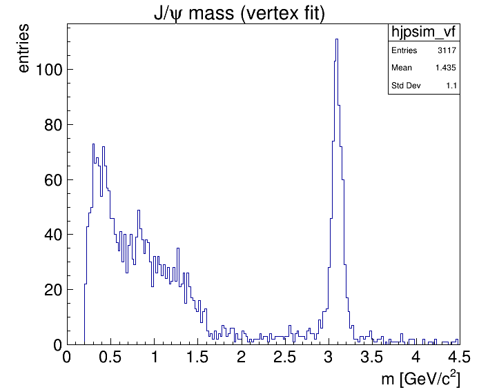
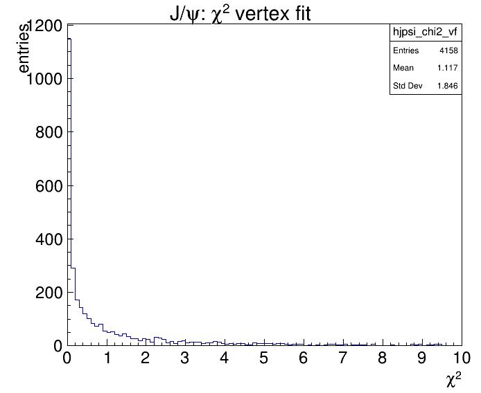
This example code shows how to access the fitted particle, the vertex and chi2 of the fit. When you try this example you may notice, that the fitted mass does not differ very much from the unfitted mass. This might be due to the fact, that the J/psi is a very short living resonance basically decaying in the IP, and the muons uncertainties are too large to be sufficiently incompatible with the origin.
This is the invariant mass distribution after the vertex fit (chi 2 < 1) and the chi2 distribution
2.5.2. Energy-Momentum-Constraint
The energy-momentum constraint fit, commonly called 4C- or 4 constraint fit, is a very powerful tool when analyzing an exclusive decay channel, i.e. reconstructing the complete event reaction, where all final state particles were reconstructed. In that case all components of the initial Lorentz vector (E, px, py, pz):sub:ini have to be conserved individually. Constraining exactly that leads to the term 4-constraint. Actually, it’s a bit of a simplification in those cases, where you want to keep all your particles on-shell (which is usually the case for final states), which somehow adds a couple of constraints as well.
However, there are two simple tools in PandaROOT to perform that kind of fit, that are called Pnd4CFitter and PndKinFitter. Since you have to bother around with daughters a lot more than in the example above, it looks a bit more complicated to use it.
// *** the lorentz vector of the initial psi(2S); important for the 4C-fit
TLorentzVector ini(0, 0, 6.231552, 7.240065);
...
  // ... in event loop ...

  // *** do 4c fit
  for (j=0;j<psi2s.GetLength();++j)
  {
    RhoKinFitter fitter(psi2s[j]); // instantiate the kin fitter in psi(2S)
    fitter.Add4MomConstraint(ini); // set 4 constraint
    fitter.Fit();                  // do the fit

    double chi2_4c = fitter.GetChi2(); // access the chi2 of the fit

    RhoCandidate *jfit = psi2s[j]->Daughter(0)->GetFit(); // access fitted cand.

    if (chi2_4c<20 && jfit)               // when good enough, fill some histos
      hjpsim_4cf->Fill(jfit->M());
  }
For the initialization of the 4C-fitter, we need the initial 4-vector _of the complete pbar p-system in addition to the candidate to be fitted. This is the only system, which is well known (for the moment without any uncertainty), and in this formation reaction it is identical with the psi(2S). It should be emphasized, that you always need to apply the 4C fit to the full exclusive system, although you are interested in improving a subresonance, like in this case the mass distribution of the J/psi. In case you don’t know by heart, how you can derive the anti-proton beam momentum necessary to generate a certain center-of-mass energy for a resonance with mass Ecm = M, the corresponding formula is p = sqrt((M4 /(4 mp 2 ) - M2 ) with the proton mass mp = 0.938272 GeV/c2.
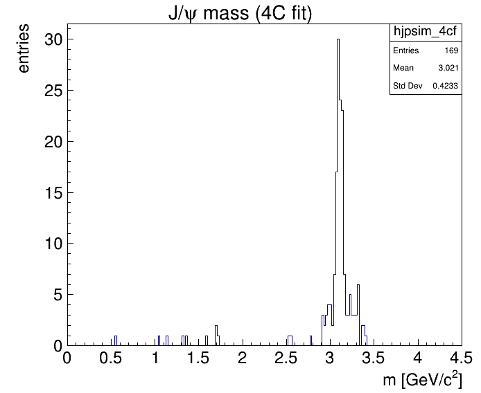
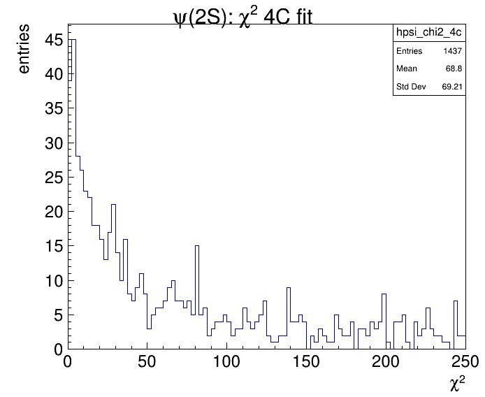
After the fit is performed, the daughters of the fitted object have to be fetched to finally compute the fitted invariant J/psi mass. When you compare the width of the reconstructed J/psi with and without this constraint, you can observe quite an improvement, although the constraint was applied to the mother of the J/psi.
This is the invariant mass distribution after the 4C fit (chi2 < 20) and the chi2 distribution:
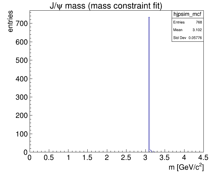
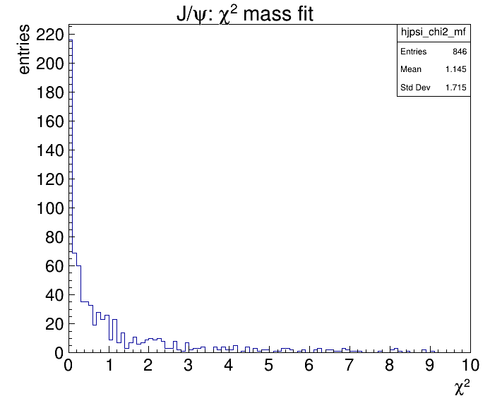
2.5.3. Mass constraint
A mass constraint fit constraints the invariant mass of the fitted 4-vector to a certain fixed value. Due to this strict constraint, it is only suitable for resonances or particles with vanishing intrinsic width, or at least a width being negligible compared to the detectors mass resolution. In PANDA context it should be fine for fitting something like D’s and J/psi’s with Gamma ≤ 100 keV, while it should not be applied for e.g. fitting the phi(1020) with a Lorentz-width of 4.3 MeV.
The most natural use case for this type of constraint is to apply it to intermediate resonances in more complex decay trees. Since we don’t have a fully working tree fitter up to now where constraints can be applied to intermediate states, the only reasonable usage in our case is to require a certain maximum value for the resulting chi2 to reduce background combinations.
In !PandaROOT one of the available classes to perform this kind of fit is e.g. PndKinFitter, where the mass constraint is applied with the AddMassConstraint method. The according code snippet looks like this:
...
  // ... in event loop ...
  // do mass constraint fit
  for (j=0;j<jpsi.GetLength();++j)
  {
    PndKinFitter mfitter(jpsi[j]);      //  instantiate fitter with J/psi
    mfitter.AddMassConstraint(3.096);   // set mass constraint to J/psi mass
    mfitter.Fit();

    double chi2m = mfitter.GetChi2();   // get the chi2 of the fit

    if (chi2m<1)
      hjpsim_mcfs->Fill(jpsi[j].M());   // fill histogram with *raw* mass
  }
As you can see we don’t even necessarily have to take a look to the fitted mass, which will in most cases anyway look like a spike at the nominal mass. However for cross-checking I would recommend to do it nevertheless.
This is the invariant mass distribution after the mass constraint fit (chi2 < 1) and the chi2 distribution:
2.5.3. Decay Tree Fitter
Ideally the complete reaction is fitted at once, taking into account all kind of constraints, like
4-vector constraint, intermediate vertex constraints, mass constraints, etc. In PandaRoot there is
such a fitter available called RhoDecayTreeFitter. The usage is fairly simple like shown in the
following example, with ini being the 4-vector of the initial pbar-p-system:
...
  // ... in event loop ...
  // do decay tree fit
  for (j=0;j<psi2s.GetLength();++j)
  {
      RhoDecayTreeFitter fittree(psi2s[j], ini);
      fittree.Fit();

      double prob_m = fittree.GetProb(); // access probability of fit

      if (prob_m > 1e-5) // when good enough, fill some histo
      {
        RhoCandidate *jfit = psi2s[j]->Daughter(0)->GetFit(); // get fitted J/psi
        hjpsim_dc->Fill(jfit->M());
    }
  }
By default, mass constraints are not set for intermediate resonances, this can be done explicitly by hand with:
fittree.setMassConstraint(psi2s[j]->Daughter(0), m0_jpsi);
where the specification of the mass (here m0_jpsi`) can be skipped optionally, if the type of the resonance is set during combinatorics, and the mass is the default mass from the TDatabasePDG. One caveat should be given: Fitting neutrals is not flawlessly working yet, so you should perhaps switch to the other fitters in that case for the time being.